data(mtcars)
mtcars$hp_z <- scale(mtcars$hp)Scaling variables in R
R
statistics
A walkthrough of a tip I recently learned
Herein I present a walkthrough of a recent improvement I made to my analyses when scaling (i.e., normalizing) variables.
Scaling or normalizing variables in R is super convenient by using the scale(x, center = TRUE, scale = TRUE) function and default arguments. Here, the variable x is mean centered and scaled to unit variance, also called a Z-score.
Let’s do this on the mtcars dataset variable hp:
Here’s proof that the newly scaled hp_z variable was indeed scaled:
library(tidyverse)
mtcars %>%
  summarise(across(contains("hp"), list(mean = mean, sd = sd))) %>%
  round(2)
hp_mean hp_sd hp_z_mean hp_z_sd
1 146.69 68.56 0 1As we can see, the M=0 and Standard Deviation(SD)=1 for hp_z.
The scale() function, however, does something really useful that I used to ignore for the longest time; it saves the scaling factors as attributes in the column/variable. This is seen in a few ways:
class(mtcars$hp_z)[1] "matrix" "array" mtcars$hp_z [,1]
[1,] -0.53509284
[2,] -0.53509284
[3,] -0.78304046
[4,] -0.53509284
[5,] 0.41294217
[6,] -0.60801861
[7,] 1.43390296
[8,] -1.23518023
[9,] -0.75387015
[10,] -0.34548584
[11,] -0.34548584
[12,] 0.48586794
[13,] 0.48586794
[14,] 0.48586794
[15,] 0.85049680
[16,] 0.99634834
[17,] 1.21512565
[18,] -1.17683962
[19,] -1.38103178
[20,] -1.19142477
[21,] -0.72469984
[22,] 0.04831332
[23,] 0.04831332
[24,] 1.43390296
[25,] 0.41294217
[26,] -1.17683962
[27,] -0.81221077
[28,] -0.49133738
[29,] 1.71102089
[30,] 0.41294217
[31,] 2.74656682
[32,] -0.54967799
attr(,"scaled:center")
[1] 146.6875
attr(,"scaled:scale")
[1] 68.56287The attribute for the mean-centering (i.e., the mean) can be accessed like this:
attr(mtcars$hp_z, "scaled:center")[1] 146.6875And the attribute for the scaling factor (i.e., the SD) can be accessed like this:
attr(mtcars$hp_z, "scaled:scale")[1] 68.56287In sum, the output of scale() is a "matrix" "array" with the centering and scaling factors, if requested, attached as attributes. Notice how they match the M and SD of the original mtcars$hp variable above.
The problem
However, there are a few issues with using scale(). The "matrix" "array" output is little annoying because it prints differently:
as_tibble(select(mtcars, mpg, contains("hp")), rownames = "car")# A tibble: 32 × 4
car mpg hp hp_z[,1]
<chr> <dbl> <dbl> <dbl>
1 Mazda RX4 21 110 -0.535
2 Mazda RX4 Wag 21 110 -0.535
3 Datsun 710 22.8 93 -0.783
4 Hornet 4 Drive 21.4 110 -0.535
5 Hornet Sportabout 18.7 175 0.413
6 Valiant 18.1 105 -0.608
7 Duster 360 14.3 245 1.43
8 Merc 240D 24.4 62 -1.24
9 Merc 230 22.8 95 -0.754
10 Merc 280 19.2 123 -0.345
# ℹ 22 more rowsand it does not play nicely with predict():
mod <- lm(mpg ~ 1 + hp_z, data = mtcars)
new_data <- data.frame(hp_z = seq(-2, 2, length.out = 100))
predict(mod, newdata = new_data, type = "response", se.fit = TRUE)
Error: variable 'hp_z' was fitted with type "nmatrix.1" but type "numeric" was suppliedIn the past, I would normally strip these features by wrapping the call with as.numeric():
mtcars$hp_zn <- as.numeric(scale(mtcars$hp))Although this will work, you lose the awesome feature of having access to the centering/scaling attributes.
The solution
I found a nice elegant solution to this issue via this Stack Overflow post.
The drop() function will drop the formatting of scale() without the loss of attributes:
mtcars$hp_z <- drop(scale(mtcars$hp)) # using drop
class(mtcars$hp_z)
[1] "numeric"as_tibble(select(mtcars, mpg, contains("hp")), rownames = "car")# A tibble: 32 × 5
car mpg hp hp_z hp_zn
<chr> <dbl> <dbl> <dbl> <dbl>
1 Mazda RX4 21 110 -0.535 -0.535
2 Mazda RX4 Wag 21 110 -0.535 -0.535
3 Datsun 710 22.8 93 -0.783 -0.783
4 Hornet 4 Drive 21.4 110 -0.535 -0.535
5 Hornet Sportabout 18.7 175 0.413 0.413
6 Valiant 18.1 105 -0.608 -0.608
7 Duster 360 14.3 245 1.43 1.43
8 Merc 240D 24.4 62 -1.24 -1.24
9 Merc 230 22.8 95 -0.754 -0.754
10 Merc 280 19.2 123 -0.345 -0.345
# ℹ 22 more rowsUsing drop() no longer causes an issue with predict():
mod <- lm(mpg ~ 1 + hp_z, data = mtcars)
new_data <- data.frame(hp_z = seq(-2, 2, length.out = 100))
pred <- predict(mod, newdata = new_data, type = "response", se.fit = TRUE)
new_data <- cbind(new_data, pred)
# plots
ggplot(new_data, aes(hp_z, fit)) +
geom_line () +
geom_ribbon(aes(ymin = fit-se.fit, ymax = fit+se.fit), alpha = 1/3) +
labs(x = "HP (in SD units)", y = "Predicted MPG", caption = "SE shading.") +
scale_x_continuous(breaks = seq(-2, 2, .5)) +
theme_bw()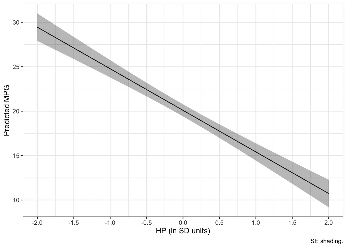
But what if we want to represent the x-axis in its original units? No problem! Just use the attributes from the scaled column to convert back to the original unstandardized units:
m <- attr(mtcars$hp_z, "scaled:center")
sd <- attr(mtcars$hp_z, "scaled:scale")
new_data$hp_o <- new_data$hp_z * sd + m

# plots
ggplot(new_data, aes(hp_o, fit)) +
  geom_line () +
  geom_ribbon(aes(ymin = fit-se.fit, ymax = fit+se.fit), alpha = 1/3) +
  labs(x = "HP (in original units)", y = "Predicted MPG", caption = "SE shading.") +
  theme_bw()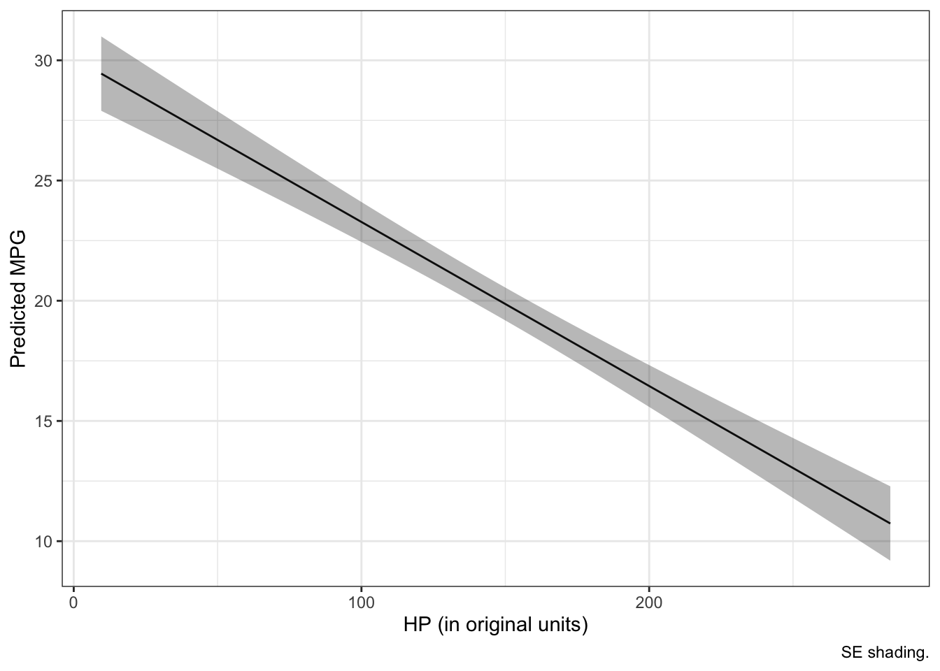
Thank you drop()!
Summary
When scaling variables in R via scale(), be sure to use the drop() function to strip away the dimensions of scale()’s output. This new variable/column will play nicely with predict() and retain the center and scale attributes for later use.